






新闻中心 
基于全色影像引导数据分布变化的高光谱全色融合网络-Pgnet
 2025-07-29
 浏览次数:次
 返回列表
返回列表本文提出基于PaddlePaddle的Pgnet网络,用于大比例(ratio=16)高光谱与全色影像融合。该网络从纠正数据分布角度,设计PDIN子网络,结合多层上采样和像素级注意力机制。通过编码器-融合-解码器框架在丰度空间处理,经多数据集实验验证,在光谱和空间保真度上表现优异,证实了数据分布变换注入细节的有效性。
☞☞☞AI 智能聊天, 问答助手, AI 智能搜索, 免费无限量使用 DeepSeek R1 模型☜☜☜

基于全色影像引导数据分布变化的高光谱全色融合网络-Pgnet-PaddlePaddle
本论文“Unmixing based PAN guided fusion network for hyperspectral imagery”基于深度学习框架PaddlePaddle来实现高光谱和全色影像融合网络—Pgnet。 该论文已发表在期刊 IEEE Transactions on Geoscience and Remote Sensing: (论文链接)
简介
高光谱和全色融合(Hyperpansharpening)指融合低空间分辨率、高光谱分辨率的高光谱影像和具有相反分辨率特征的全色影像来获得同时具有高空间、光谱分辨率的高光谱影像。由于两幅输入影像分辨率差异过大,该融合问题非常病态。而现有的融合方法大都关注于小比例融合,缺乏实用性。所以本文关注于大比例融合任务(ratio=16),并通过所设计的网络有效的注入空间细节,极大地缓解了该问题的病态性。
本文的融合方法首次从纠正数据分布的角度出发,即设计具有可解释性的细节注入子网络—PDIN,并利用多层上采样和像素级注意力机制来融合两幅影像。总体融合框架如下所示:
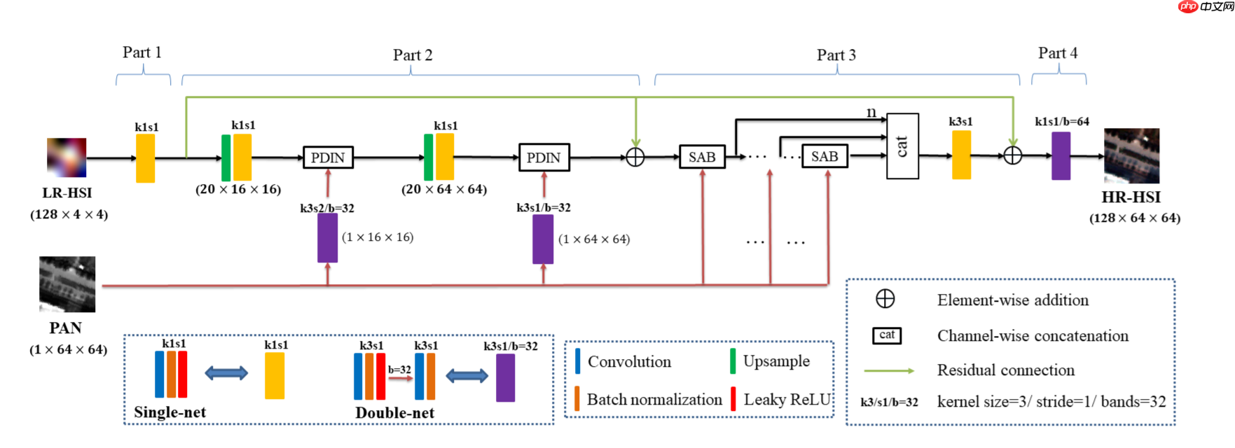
通过解混高光谱影像得到的丰度和端元可以以低复杂度和高精度来表达源影像,已经被广泛采用在高光谱处理领域。本文的融合过程是在丰度空间中进行的。采用自编码器的思想,即通过了编码到丰度(Part 1)—融合(Part 2,3)—解码到融合影像(Part 4)的过程。
PDIN
通过公式推导和模拟实验,我们得到了高光谱影像投影后的丰度和全色强度之间的线性、非线性关系。
线性关系
X=EA+NX ——光谱解混模型,高光谱X可以分解为端元E和丰度A,NX为噪声。
P=SX+NP ——全色为高光谱影像的线性组合,P为全色影像, S为光谱响应函数。
将上述两公式结合:
==>P=SEA+SNX+NP
==>P=S’A+N’ ——其中S’=SE,N’=SNX+NP
P为全色强度,A为高光谱影像投影后的丰度,S’为光谱响应函数,N’为噪声,
可以看出全色为丰度的线性组合,即二者为线性相关。
非线性关系
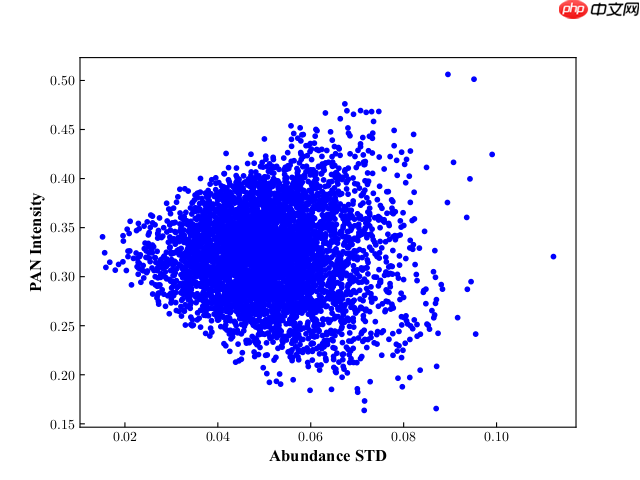
该非线性关系通过模拟实验得到,即通过从USGS光谱库中选择纯净光谱端元来构建模拟高光谱和全色数据,然后绘制模拟数据的丰度标准差和全色强度之间的散点分布图如上图所示。
上图所示为接近正确的分布,但实际在网络前向传播过程中,一些模块如上采样模块生成的数据分布并不正确,我们的想法是通过调整丰度数据的分布来变相的注入全色细节。该调整过程设想如下图:
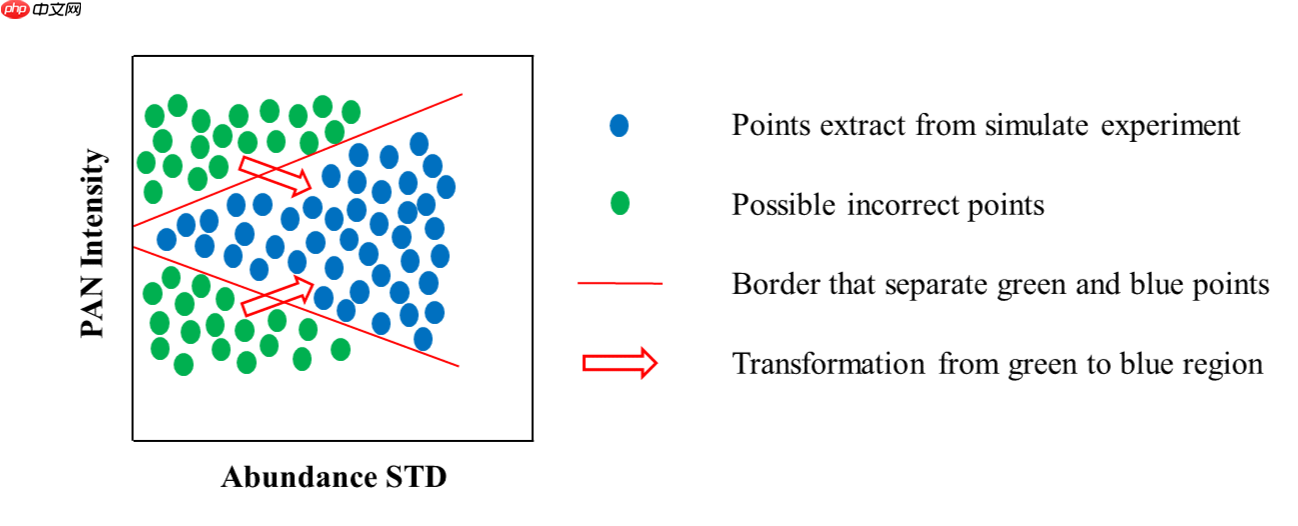
如图所示,绿点代表了可能的不正确的像元(在前向传播过程中生成),蓝点代表了符合正确分布的点,红色箭头代表了我们想要完成的数据分布变换操作,即将绿点变换到蓝点区域。
 Motiff妙多
Motiff妙多是一款AI驱动的界面设计工具,定位为“AI时代设计工具”
 334
查看详情
334
查看详情

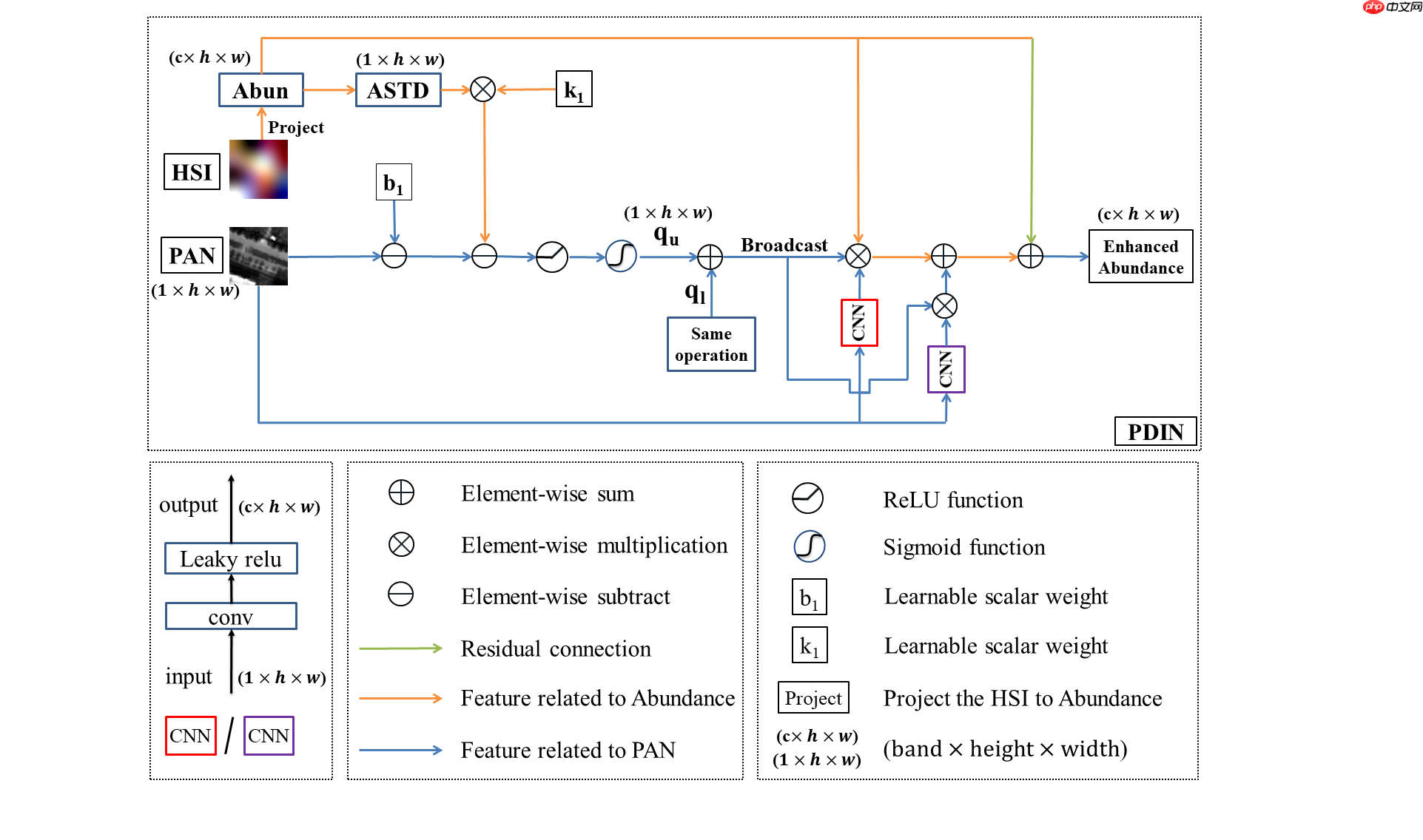
该变换通过改变绿点像元的标准差来进行,即图中坐标横轴,把每个像元乘以特定的权重来移动到蓝点区域。值得注意的是,纵轴(全色强度)可以看成是一种约束或监督,即在变换过程中其对应的全色强度应保持不变。具体的推导过程篇幅较长故未写出,详细部分可以看论文。下面是所提出的全色细节注入子网络结构(PDIN):
# 模拟实验代码,运行可以得到非线性的散点分布图,由于每次丰度随机生成,故形状会稍微有所差异.import numpy as npimport matplotlib.pyplot as plt
srf_pan = np.load('/home/aistudio/data/data124050/srf_pan.npy')

filename = '/home/aistudio/work/file/envi_plot3.txt'curve_data =np.loadtxt(filename, skiprows=13)[:, 1:]

pixel_num = 5000abun = np.random.rand(pixel_num, curve_data.shape[1])
abun_sum = np.sum(abun, axis=1)
abun = abun / np.expand_dims(abun_sum, axis=1)

intensity = np.dot(srf_pan, np.dot(curve_data[:, :], np.transpose(abun))[:srf_pan.shape[0], :]) / np.sum(srf_pan)
x_var = np.std(abun, axis=1)    # 每个像元端元丰度的标准差plt.scatter(x_var, intensity, color='b', s=10)
plt.xlabel('Abundance STD')
plt.ylabel('PAN Intensity')
plt.show()
<Figure size 432x288 with 1 Axes>
网络框架
Part 1:
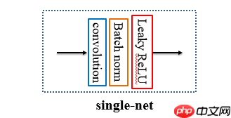
第一部分为编码器,即将高光谱影像投影到丰度空间。采用了标准的Conv+BN+Lrelu结构. 丰度的特征波段通过后续实验选择为20.
Part 2:
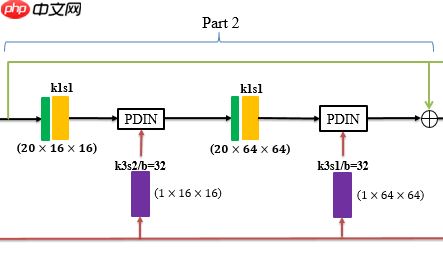

该Part为上采样模块,其中紫色为连续两次卷积block,绿色为上采样block,包括bicubic内插和单卷积。绿色箭头为残差连接。黑色箭头代表丰度特征,红色箭头代表全色特征。因本文关注大比例融合任务,故采用两次上采样来进一步提高性能。
Part 3:
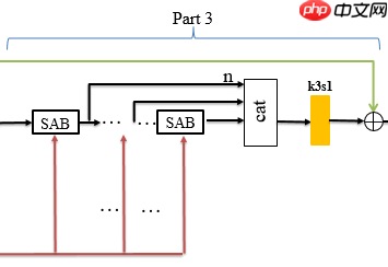
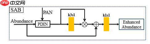
如图所示,第三部分采用了联级的注意力机制,并再次在每个注意力block中使用了PDIN来注入细节.黄色模块为Part 1的single-net.
Part 4:
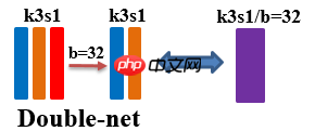
第四部分为解码器,将丰度解码到高光谱影像空间。这里的卷积操作相当于将丰度乘以端元(卷积核参数)得到高光谱影像(线性混合模型)。
In [3]#请运行此代码以进行训练,默认500epoch,如需改变训练epoch和其他训练细节,请进入main和其他文件中进行修改。!python /home/aistudio/work/code/main_all.py
/opt/conda/envs/python35-paddle120-env/lib/python3.7/site-packages/paddle/fluid/layers/utils.py:26: DeprecationWarning: `np.int` is a deprecated alias for the builtin `int`. To silence this warning, use `int` by itself. Doing this will not modify any beh*ior and is safe. When replacing `np.int`, you may wish to use e.g. `np.int64` or `np.int32` to specify the precision. If you wish to review your current use, check the release note link for additional information.
Deprecated in NumPy 1.20; for more details and guidance: https://numpy.org/devdocs/release/1.20.0-notes.html#deprecations
def convert_to_list(value, n, name, dtype=np.int):
Namespace(batch_size=15, dataset='JiaXing', endmember=20, in_nc=126, load_para=False, lr=0.002, model='Pgnet', momentum=0.05, num_epochs=500, resume='', start_epoch=1, step=100, test=False, test_batch_size=1)
original_msi.shape: (126, 1024, 12480)
max value: 0.9999695
W0218 19:02:59.614563 470 device_context.cc:362] Please NOTE: device: 0, GPU Compute Capability: 7.0, Driver API Version: 10.1, Runtime API Version: 10.1
W0218 19:02:59.619832 470 device_context.cc:372] device: 0, cuDNN Version: 7.6.
[1, 126, 64, 780]
blur_data.shape:(126, 64, 780)
temp_pan.shape:(1, 1024, 12480)
croping train images...
(126, 64, 624)
(1, 1024, 9984)
(126, 1024, 9984)
size of train_hrpanimage:(1098, 1, 64, 64) train_lrhsimage:(1098, 126, 4, 4) train_label:(1098, 126, 64, 64)
croping test images...
(126, 64, 156)
(1, 1024, 2496)
(126, 1024, 2496)
size of test_hrpanimage:(9, 1, 256, 256) test_lrhsimage:(9, 126, 16, 16) test_label:(9, 126, 256, 256)
train size:(1098, 1, 64, 64)
test size:(9, 1, 256, 256)
16
(1098, 126, 4, 4)
(9, 126, 16, 16)
/opt/conda/envs/python35-paddle120-env/lib/python3.7/site-packages/paddle/nn/layer/conv.py:83: DeprecationWarning: `np.int` is a deprecated alias for the builtin `int`. To silence this warning, use `int` by itself. Doing this will not modify any beh*ior and is safe. When replacing `np.int`, you may wish to use e.g. `np.int64` or `np.int32` to specify the precision. If you wish to review your current use, check the release note link for additional information.
Deprecated in NumPy 1.20; for more details and guidance: https://numpy.org/devdocs/release/1.20.0-notes.html#deprecations
} and not isinstance(padding, np.int):
Total number of paramerters in networks is Tensor(shape=[1], dtype=int64, place=CUDAPlace(0), stop_gradient=False,
[49100])
/opt/conda/envs/python35-paddle120-env/lib/python3.7/site-packages/paddle/fluid/dataloader/dataloader_iter.py:89: DeprecationWarning: `np.bool` is a deprecated alias for the builtin `bool`. To silence this warning, use `bool` by itself. Doing this will not modify any beh*ior and is safe. If you specifically wanted the numpy scalar type, use `np.bool_` here.
Deprecated in NumPy 1.20; for more details and guidance: https://numpy.org/devdocs/release/1.20.0-notes.html#deprecations
if isinstance(slot[0], (np.ndarray, np.bool, numbers.Number)):
/opt/conda/envs/python35-paddle120-env/lib/python3.7/site-packages/paddle/nn/layer/norm.py:648: UserWarning: When training, we now always track global mean and variance.
"When training, we now always track global mean and variance.")
epoch 10 of 500, using time: 7.06 , loss of train: 1.0242
epoch 20 of 500, using time: 7.16 , loss of train: 0.1000
epoch 30 of 500, using time: 7.40 , loss of train: 0.0981
epoch 40 of 500, using time: 7.06 , loss of train: 0.0954
epoch 50 of 500, using time: 7.10 , loss of train: 0.0954
epoch 60 of 500, using time: 7.25 , loss of train: 0.0943
epoch 70 of 500, using time: 7.16 , loss of train: 0.0919
epoch 80 of 500, using time: 7.21 , loss of train: 0.0914
epoch 90 of 500, using time: 7.13 , loss of train: 0.0925
 epoch 100 of 500, using time: 7.18 , loss of train: 0.0924
epoch 110 of 500, using time: 7.14 , loss of train: 0.0885
epoch 120 of 500, using time: 7.20 , loss of train: 0.0895
epoch 130 of 500, using time: 7.16 , loss of train: 0.0901
epoch 140 of 500, using time: 7.08 , loss of train: 0.0889
epoch 150 of 500, using time: 7.26 , loss of train: 0.0893
epoch 160 of 500, using time: 7.08 , loss of train: 0.0894
epoch 170 of 500, using time: 7.26 , loss of train: 0.0885
epoch 180 of 500, using time: 7.23 , loss of train: 0.0875
epoch 190 of 500, using time: 7.11 , loss of train: 0.0892
epoch 200 of 500, using time: 7.22 , loss of train: 0.0882
epoch 210 of 500, using time: 7.15 , loss of train: 0.0890
epoch 220 of 500, using time: 7.05 , loss of train: 0.0874
epoch 230 of 500, using time: 7.20 , loss of train: 0.0888
epoch 240 of 500, using time: 7.23 , loss of train: 0.0877
epoch 250 of 500, using time: 7.03 , loss of train: 0.0892
epoch 260 of 500, using time: 7.15 , loss of train: 0.0896
epoch 270 of 500, using time: 7.18 , loss of train: 0.0884
epoch 280 of 500, using time: 7.07 , loss of train: 0.0883
epoch 290 of 500, using time: 7.15 , loss of train: 0.0889
epoch 300 of 500, using time: 7.15 , loss of train: 0.0905
epoch 310 of 500, using time: 7.38 , loss of train: 0.0884
epoch 320 of 500, using time: 7.45 , loss of train: 0.0896
epoch 330 of 500, using time: 7.08 , loss of train: 0.0892
epoch 340 of 500, using time: 7.00 , loss of train: 0.0900
epoch 350 of 500, using time: 7.16 , loss of train: 0.0884
epoch 360 of 500, using time: 7.06 , loss of train: 0.0897
epoch 370 of 500, using time: 7.17 , loss of train: 0.0890
epoch 380 of 500, using time: 7.34 , loss of train: 0.0880
epoch 390 of 500, using time: 7.21 , loss of train: 0.0886
epoch 400 of 500, using time: 7.11 , loss of train: 0.0883
epoch 410 of 500, using time: 7.05 , loss of train: 0.0888
epoch 420 of 500, using time: 7.02 , loss of train: 0.0876
epoch 430 of 500, using time: 7.03 , loss of train: 0.0882
epoch 440 of 500, using time: 7.06 , loss of train: 0.0879
epoch 450 of 500, using time: 7.04 , loss of train: 0.0892
epoch 460 of 500, using time: 7.03 , loss of train: 0.0879
epoch 470 of 500, using time: 7.08 , loss of train: 0.0875
epoch 480 of 500, using time: 6.98 , loss of train: 0.0890
epoch 490 of 500, using time: 7.07 , loss of train: 0.0882
epoch 500 of 500, using time: 7.04 , loss of train: 0.0878
################## reference comparision #######################
metrics: PSNR, SSIM, SAM, ERGAS, SCC, Q, RMSE
Pf [36.4348, 0.9156, 0.0632, 0.5868, 0.8875, 0.4684, 0.0151]
################## reference comparision #######################
epoch 100 of 500, using time: 7.18 , loss of train: 0.0924
epoch 110 of 500, using time: 7.14 , loss of train: 0.0885
epoch 120 of 500, using time: 7.20 , loss of train: 0.0895
epoch 130 of 500, using time: 7.16 , loss of train: 0.0901
epoch 140 of 500, using time: 7.08 , loss of train: 0.0889
epoch 150 of 500, using time: 7.26 , loss of train: 0.0893
epoch 160 of 500, using time: 7.08 , loss of train: 0.0894
epoch 170 of 500, using time: 7.26 , loss of train: 0.0885
epoch 180 of 500, using time: 7.23 , loss of train: 0.0875
epoch 190 of 500, using time: 7.11 , loss of train: 0.0892
epoch 200 of 500, using time: 7.22 , loss of train: 0.0882
epoch 210 of 500, using time: 7.15 , loss of train: 0.0890
epoch 220 of 500, using time: 7.05 , loss of train: 0.0874
epoch 230 of 500, using time: 7.20 , loss of train: 0.0888
epoch 240 of 500, using time: 7.23 , loss of train: 0.0877
epoch 250 of 500, using time: 7.03 , loss of train: 0.0892
epoch 260 of 500, using time: 7.15 , loss of train: 0.0896
epoch 270 of 500, using time: 7.18 , loss of train: 0.0884
epoch 280 of 500, using time: 7.07 , loss of train: 0.0883
epoch 290 of 500, using time: 7.15 , loss of train: 0.0889
epoch 300 of 500, using time: 7.15 , loss of train: 0.0905
epoch 310 of 500, using time: 7.38 , loss of train: 0.0884
epoch 320 of 500, using time: 7.45 , loss of train: 0.0896
epoch 330 of 500, using time: 7.08 , loss of train: 0.0892
epoch 340 of 500, using time: 7.00 , loss of train: 0.0900
epoch 350 of 500, using time: 7.16 , loss of train: 0.0884
epoch 360 of 500, using time: 7.06 , loss of train: 0.0897
epoch 370 of 500, using time: 7.17 , loss of train: 0.0890
epoch 380 of 500, using time: 7.34 , loss of train: 0.0880
epoch 390 of 500, using time: 7.21 , loss of train: 0.0886
epoch 400 of 500, using time: 7.11 , loss of train: 0.0883
epoch 410 of 500, using time: 7.05 , loss of train: 0.0888
epoch 420 of 500, using time: 7.02 , loss of train: 0.0876
epoch 430 of 500, using time: 7.03 , loss of train: 0.0882
epoch 440 of 500, using time: 7.06 , loss of train: 0.0879
epoch 450 of 500, using time: 7.04 , loss of train: 0.0892
epoch 460 of 500, using time: 7.03 , loss of train: 0.0879
epoch 470 of 500, using time: 7.08 , loss of train: 0.0875
epoch 480 of 500, using time: 6.98 , loss of train: 0.0890
epoch 490 of 500, using time: 7.07 , loss of train: 0.0882
epoch 500 of 500, using time: 7.04 , loss of train: 0.0878
################## reference comparision #######################
metrics: PSNR, SSIM, SAM, ERGAS, SCC, Q, RMSE
Pf [36.4348, 0.9156, 0.0632, 0.5868, 0.8875, 0.4684, 0.0151]
################## reference comparision #######################
 epoch 100 of 500, using time: 7.18 , loss of train: 0.0924
epoch 110 of 500, using time: 7.14 , loss of train: 0.0885
epoch 120 of 500, using time: 7.20 , loss of train: 0.0895
epoch 130 of 500, using time: 7.16 , loss of train: 0.0901
epoch 140 of 500, using time: 7.08 , loss of train: 0.0889
epoch 150 of 500, using time: 7.26 , loss of train: 0.0893
epoch 160 of 500, using time: 7.08 , loss of train: 0.0894
epoch 170 of 500, using time: 7.26 , loss of train: 0.0885
epoch 180 of 500, using time: 7.23 , loss of train: 0.0875
epoch 190 of 500, using time: 7.11 , loss of train: 0.0892
epoch 200 of 500, using time: 7.22 , loss of train: 0.0882
epoch 210 of 500, using time: 7.15 , loss of train: 0.0890
epoch 220 of 500, using time: 7.05 , loss of train: 0.0874
epoch 230 of 500, using time: 7.20 , loss of train: 0.0888
epoch 240 of 500, using time: 7.23 , loss of train: 0.0877
epoch 250 of 500, using time: 7.03 , loss of train: 0.0892
epoch 260 of 500, using time: 7.15 , loss of train: 0.0896
epoch 270 of 500, using time: 7.18 , loss of train: 0.0884
epoch 280 of 500, using time: 7.07 , loss of train: 0.0883
epoch 290 of 500, using time: 7.15 , loss of train: 0.0889
epoch 300 of 500, using time: 7.15 , loss of train: 0.0905
epoch 310 of 500, using time: 7.38 , loss of train: 0.0884
epoch 320 of 500, using time: 7.45 , loss of train: 0.0896
epoch 330 of 500, using time: 7.08 , loss of train: 0.0892
epoch 340 of 500, using time: 7.00 , loss of train: 0.0900
epoch 350 of 500, using time: 7.16 , loss of train: 0.0884
epoch 360 of 500, using time: 7.06 , loss of train: 0.0897
epoch 370 of 500, using time: 7.17 , loss of train: 0.0890
epoch 380 of 500, using time: 7.34 , loss of train: 0.0880
epoch 390 of 500, using time: 7.21 , loss of train: 0.0886
epoch 400 of 500, using time: 7.11 , loss of train: 0.0883
epoch 410 of 500, using time: 7.05 , loss of train: 0.0888
epoch 420 of 500, using time: 7.02 , loss of train: 0.0876
epoch 430 of 500, using time: 7.03 , loss of train: 0.0882
epoch 440 of 500, using time: 7.06 , loss of train: 0.0879
epoch 450 of 500, using time: 7.04 , loss of train: 0.0892
epoch 460 of 500, using time: 7.03 , loss of train: 0.0879
epoch 470 of 500, using time: 7.08 , loss of train: 0.0875
epoch 480 of 500, using time: 6.98 , loss of train: 0.0890
epoch 490 of 500, using time: 7.07 , loss of train: 0.0882
epoch 500 of 500, using time: 7.04 , loss of train: 0.0878
################## reference comparision #######################
metrics: PSNR, SSIM, SAM, ERGAS, SCC, Q, RMSE
Pf [36.4348, 0.9156, 0.0632, 0.5868, 0.8875, 0.4684, 0.0151]
################## reference comparision #######################
epoch 100 of 500, using time: 7.18 , loss of train: 0.0924
epoch 110 of 500, using time: 7.14 , loss of train: 0.0885
epoch 120 of 500, using time: 7.20 , loss of train: 0.0895
epoch 130 of 500, using time: 7.16 , loss of train: 0.0901
epoch 140 of 500, using time: 7.08 , loss of train: 0.0889
epoch 150 of 500, using time: 7.26 , loss of train: 0.0893
epoch 160 of 500, using time: 7.08 , loss of train: 0.0894
epoch 170 of 500, using time: 7.26 , loss of train: 0.0885
epoch 180 of 500, using time: 7.23 , loss of train: 0.0875
epoch 190 of 500, using time: 7.11 , loss of train: 0.0892
epoch 200 of 500, using time: 7.22 , loss of train: 0.0882
epoch 210 of 500, using time: 7.15 , loss of train: 0.0890
epoch 220 of 500, using time: 7.05 , loss of train: 0.0874
epoch 230 of 500, using time: 7.20 , loss of train: 0.0888
epoch 240 of 500, using time: 7.23 , loss of train: 0.0877
epoch 250 of 500, using time: 7.03 , loss of train: 0.0892
epoch 260 of 500, using time: 7.15 , loss of train: 0.0896
epoch 270 of 500, using time: 7.18 , loss of train: 0.0884
epoch 280 of 500, using time: 7.07 , loss of train: 0.0883
epoch 290 of 500, using time: 7.15 , loss of train: 0.0889
epoch 300 of 500, using time: 7.15 , loss of train: 0.0905
epoch 310 of 500, using time: 7.38 , loss of train: 0.0884
epoch 320 of 500, using time: 7.45 , loss of train: 0.0896
epoch 330 of 500, using time: 7.08 , loss of train: 0.0892
epoch 340 of 500, using time: 7.00 , loss of train: 0.0900
epoch 350 of 500, using time: 7.16 , loss of train: 0.0884
epoch 360 of 500, using time: 7.06 , loss of train: 0.0897
epoch 370 of 500, using time: 7.17 , loss of train: 0.0890
epoch 380 of 500, using time: 7.34 , loss of train: 0.0880
epoch 390 of 500, using time: 7.21 , loss of train: 0.0886
epoch 400 of 500, using time: 7.11 , loss of train: 0.0883
epoch 410 of 500, using time: 7.05 , loss of train: 0.0888
epoch 420 of 500, using time: 7.02 , loss of train: 0.0876
epoch 430 of 500, using time: 7.03 , loss of train: 0.0882
epoch 440 of 500, using time: 7.06 , loss of train: 0.0879
epoch 450 of 500, using time: 7.04 , loss of train: 0.0892
epoch 460 of 500, using time: 7.03 , loss of train: 0.0879
epoch 470 of 500, using time: 7.08 , loss of train: 0.0875
epoch 480 of 500, using time: 6.98 , loss of train: 0.0890
epoch 490 of 500, using time: 7.07 , loss of train: 0.0882
epoch 500 of 500, using time: 7.04 , loss of train: 0.0878
################## reference comparision #######################
metrics: PSNR, SSIM, SAM, ERGAS, SCC, Q, RMSE
Pf [36.4348, 0.9156, 0.0632, 0.5868, 0.8875, 0.4684, 0.0151]
################## reference comparision #######################实验结果
实验部分,通过选择四个数据集进行了模拟和真实实验。模拟实验数据集包括JiaXing, chikusei 和 XiongAn。真实实验数据集包括Real dataset. 此外,为了验证网络在小比例融合任务上的泛化性能,我们进行了ratio 4 和 8的实验。消融实验也被设计来验证各个网络模块的必要性和分布变化规律的正确性,即在PDIN中,通过改变数据分布来注入空间细节并不只是设想,实验结果证实了模拟实验所提出的假设。
JiaXing 实验结果: 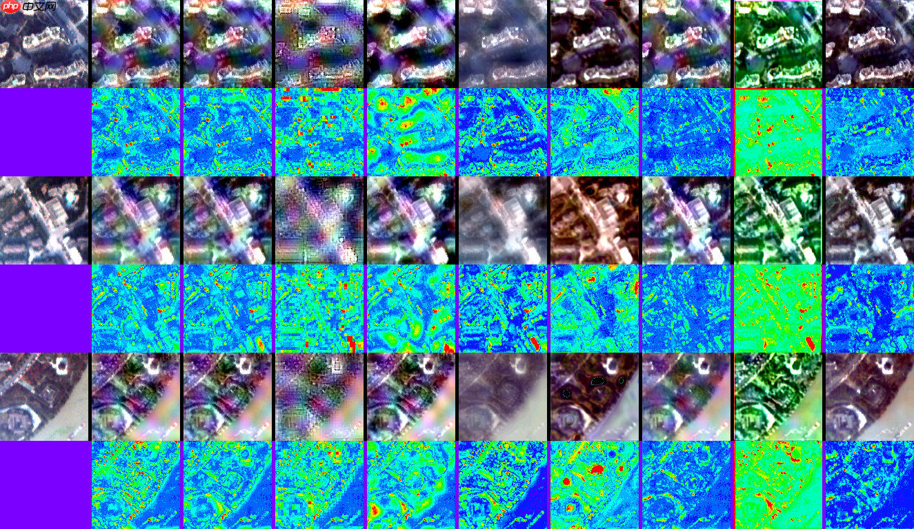
其中第一列为真实影像,后续每列为各个方法的结果,本文方法在最后一列。奇数行为融合高光谱,偶数行是和真值的差值。
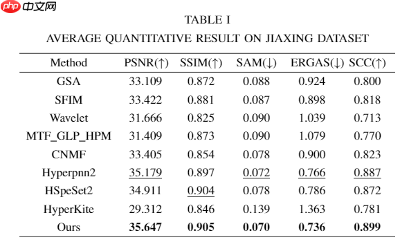
从上述实验结果可以看出,相比于其他方法,本文方法展现出了更好的光谱和空间保真度。包括多个指标的定量结果也表明我们的方法取得了最高的性能。由于空间关系,其他三个数据集的结果并未展现,但我们的方法均取得了最好的结果。
数据分布变换假设的验证
为了验证提出的PDIN对于数据分布变换的效果,我们对测试影像的中间结果进行了分析,结果如下: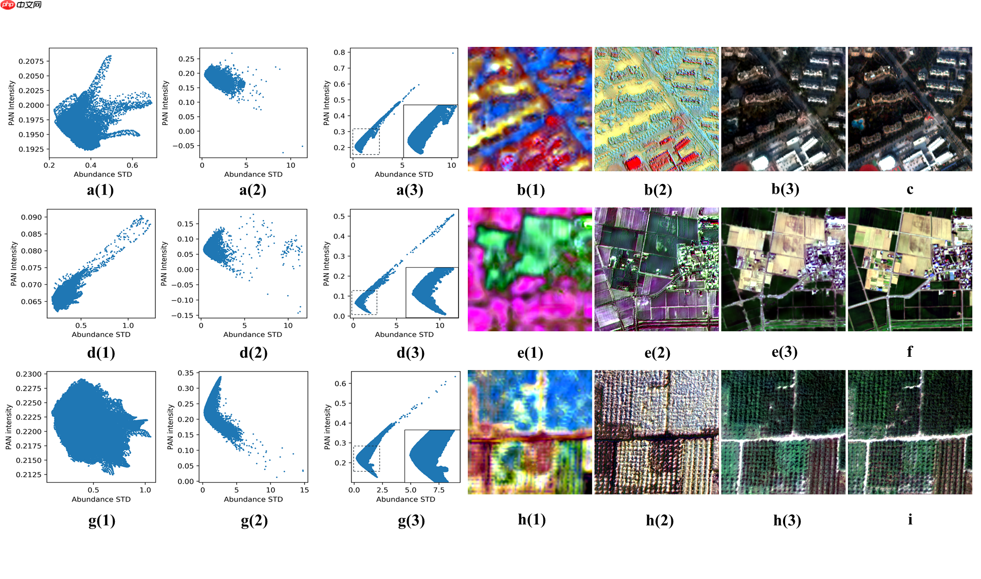 每行代表不同的数据集,以第一行JiaXing数据为例,前三个中间结果散点图(横轴为丰度标准差,纵轴为全色强度)分别代表第二个上采样block后、第二个PDIN后和Part 3的末端。第四到六幅影像为对应解码得到的高光谱影像,最后一个为真实影像。从第一列到第二列,即经过了一次PDIN的细节注入后,数据分布变得些许像模拟数据的分布了,对应的高光谱影像质量也有所提升。在经过了带有PDIN的注意力机制后,即第三列,数据分布变成了和模拟数据几乎相等的分布,对应的高光谱质量也和真实影像非常接近。验证了PDIN能够通过改变数据分布来注入细节和提升影像质量。
以上就是基于全色影像引导数据分布变化的高光谱全色融合网络-Pgnet的详细内容,更多请关注其它相关文章!
# python
# 过程中
# 建设手机网站价格
# 平度电商网站建设
# 关于推广营销说说心情
# 沙田网站优化哪些服务
# 石家庄网站推广业务公司
# 营销推广方法都有哪些
# 山东seo外包多少钱
# 导航优化网站建设
# 岳阳seo优化批发
# 如何开网站广告语推广
# 第二个
# 两次
# 进行了
# 标准差
# 纵轴
# 所示
# 一言
# 中文网
# type
# fig
# udio
# 子网
# ai
相关栏目:
【
行业资讯67740 】
【
技术百科0 】
【
网络运营39195 】
相关推荐:
4800日元等于多少人民币
kingston是什么_kingston是什么意思
苹果16系统有哪些问题
远程桌面如何发送命令
充电器上的power是什么意思
如何辨别固态硬盘坏块
j*a map数组怎么取值
征信信誉不好如何恢复 如何修复不良征信方法
为什么ai老是说链接面板中缺少某些文件
华为交换机如何复制命令行
43寸电视长宽多少厘米
怎么在typescript写原型链
华为5g手机掉了怎么定位找回
语音聊天软件哪个好 语音聊天软件2025排行榜
为什么夸克书架书单没了
unix时间戳转换公式
如何寻找和修复无法在 AI 中找到文件的问题
单片机蜂鸣器响了怎么停
系统如何装在固态硬盘
春运抢票需要抢几天
命令行如何启动应用程序
光猫power灯一直闪是什么意思
typescript怎么使用map
如何清理固态硬盘
juice是什么意思
征信信用不好如何恢复 征信信用不好如何恢复指南
ftp$如何执行宏命令
折叠屏手机好不好,耐不耐用
如何用chown命令
得物上怎么样申请退换货 得物上退换货详细指南(包含海外)
命令行如何打开文件
j*a怎么用数组缓存
哪个品牌有折叠屏手机卖
笔记本如何选择固态硬盘
摄像机的power chg是什么意思中文
win7如何打开命令行窗口
如何使用ping命令
单片机速度怎么看
如何激活固态硬盘
什么是夸克模组文件格式
高市盈率是什么意思
typescript如何标记私有方法
单片机.lib文件怎么打开
固态硬盘损坏如何修复
硬盘和固态硬盘如何区分
如何去除计算器的命令
三星 nfc什么功能是什么意思
j*a怎么声明byte数组
公司的tm市盈率为负是什么意思
苹果16有哪些改善
